Karolina's Bioinformatics Portfolio
View the Project on GitHub akn006-navarro/bimm143_github_redo
Class 09, Candy Data!
Karolina Navarro (A19106745)
- Background
- Data Import
- Exploratory Analysis
- Overall Candy Rankings
- Taking a look at priceprint
- Exploring the correlation data
- PCA
Background
In this mini project, you will explore FiveThirtyEight’s Halloween Candy data set
We will use lots of gglpot some basic stats, correlation analysis and PCA to make sense of the landscape of US candy - something hopefully more relatable than the proteomics and transcriptomics
Data Import
candy_file <- read.csv("candy-data.csv", row.names = 1)
head(candy_file)
             chocolate fruity caramel peanutyalmondy nougat crispedricewafer
100 Grand            1      0       1              0      0                1
3 Musketeers         1      0       0              0      1                0
One dime             0      0       0              0      0                0
One quarter          0      0       0              0      0                0
Air Heads            0      1       0              0      0                0
Almond Joy           1      0       0              1      0                0
             hard bar pluribus sugarpercent pricepercent winpercent
100 Grand       0   1        0        0.732        0.860   66.97173
3 Musketeers    0   1        0        0.604        0.511   67.60294
One dime        0   0        0        0.011        0.116   32.26109
One quarter     0   0        0        0.011        0.511   46.11650
Air Heads       0   0        0        0.906        0.511   52.34146
Almond Joy      0   1        0        0.465        0.767   50.34755
Q1. How many different candy types are in this dataset?
nrow(candy_file)
[1] 85
Q2. How many fruity candy types are in the dataset?
sum(candy_file$fruity)
[1] 38
Q.3 What is your favorite candy (other than Twix) in the dataset and what is it’s winpercent value?
library(dplyr)
Attaching package: 'dplyr'

The following objects are masked from 'package:stats':

    filter, lag

The following objects are masked from 'package:base':

    intersect, setdiff, setequal, union
candy_file |>
  filter(row.names(candy_file)=="Mike & Ike") |>
  select(winpercent)
           winpercent
Mike & Ike   46.41172
Q4. What is the winpercent value for “Kit Kat”?
candy_file["Kit Kat", "winpercent"]
[1] 76.7686
Q5. What is the winpercent value for “Tootsie Roll Snack Bars”?
candy_file["Tootsie Roll Snack Bars", "winpercent"]
[1] 49.6535
Q6. Is there any variable/column that looks to be on a different scale to the majority of the other columns in the dataset?
Yes!
Q7. What do you think a zero and one represent for the
candy$chocolatecolumn?
1 means constains chocolate 0 means it does not contain any chocolate
Exploratory Analysis
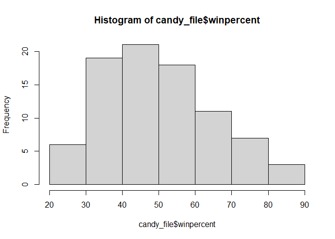
Q8. Plot a histogram of winpercent values
hist(candy_file$winpercent)
library(ggplot2)


ggplot(candy_file) +
  aes(x = winpercent) +
  geom_histogram(bins = 14, col="pink", ) + theme_bw()
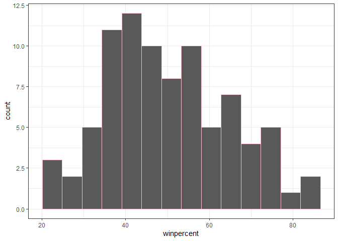
Q9. Is the distribution of winpercent values symmetrical?
No!
Q10. Is the center of the distribution above or below 50%?
Below
summary(candy_file$winpercent)
   Min. 1st Qu.  Median    Mean 3rd Qu.    Max.
  22.45   39.14   47.83   50.32   59.86   84.18
Q11. On average is chocolate candy higher or lower ranked than fruit candy?
- Find all chocolate candy
- Get their winpercent values
- Find the mean
- Find all fruity candy 5.Get their winpercent values 6.Find the mean 7.Compare the two
candy_file$chocolate == 1
 [1]  TRUE  TRUE FALSE FALSE FALSE  TRUE  TRUE FALSE FALSE FALSE  TRUE FALSE
[13] FALSE FALSE FALSE FALSE FALSE FALSE FALSE FALSE FALSE FALSE  TRUE  TRUE
[25]  TRUE  TRUE FALSE  TRUE  TRUE FALSE FALSE FALSE  TRUE  TRUE FALSE  TRUE
[37]  TRUE  TRUE  TRUE  TRUE  TRUE FALSE  TRUE  TRUE FALSE FALSE FALSE  TRUE
[49] FALSE FALSE FALSE  TRUE  TRUE  TRUE  TRUE FALSE  TRUE FALSE FALSE  TRUE
[61] FALSE FALSE  TRUE FALSE  TRUE  TRUE FALSE FALSE FALSE FALSE FALSE FALSE
[73] FALSE FALSE  TRUE  TRUE  TRUE  TRUE FALSE  TRUE FALSE FALSE FALSE FALSE
[85]  TRUE
choc.candy <- candy_file[candy_file$chocolate == 1,]
choc.win <- choc.candy$winpercent
mean(choc.win)
[1] 60.92153
fruit.win <- candy_file[candy_file$fruity == 1,]$winpercent
mean(fruit.win)
[1] 44.11974
Q12. Is this difference statistically significant?
t.test(choc.win, fruit.win)
    Welch Two Sample t-test

data:  choc.win and fruit.win
t = 6.2582, df = 68.882, p-value = 2.871e-08
alternative hypothesis: true difference in means is not equal to 0
95 percent confidence interval:
 11.44563 22.15795
sample estimates:
mean of x mean of y
 60.92153  44.11974
We can reject the null and accept the alternate, and report that there is stastical significance considering the p value that is less than 0.05.
Overall Candy Rankings
Q13. What are the five least liked candy types in this set?
y <- c("y", "a", "z")
sort(y)
[1] "a" "y" "z"
y
[1] "y" "a" "z"
order(y)
[1] 2 1 3
ord.ind <- order(candy_file$winpercent)
head(candy_file[ord.ind, ], 5)
                   chocolate fruity caramel peanutyalmondy nougat
Nik L Nip                  0      1       0              0      0
Boston Baked Beans         0      0       0              1      0
Chiclets                   0      1       0              0      0
Super Bubble               0      1       0              0      0
Jawbusters                 0      1       0              0      0
                   crispedricewafer hard bar pluribus sugarpercent pricepercent
Nik L Nip                         0    0   0        1        0.197        0.976
Boston Baked Beans                0    0   0        1        0.313        0.511
Chiclets                          0    0   0        1        0.046        0.325
Super Bubble                      0    0   0        0        0.162        0.116
Jawbusters                        0    1   0        1        0.093        0.511
                   winpercent
Nik L Nip            22.44534
Boston Baked Beans   23.41782
Chiclets             24.52499
Super Bubble         27.30386
Jawbusters           28.12744
Q14. What are the top 5 all time favorite candy types out of this set?
ord.ind <- order(candy_file$winpercent)
tail(candy_file[ord.ind, ], 5)
                          chocolate fruity caramel peanutyalmondy nougat
Snickers                          1      0       1              1      1
Kit Kat                           1      0       0              0      0
Twix                              1      0       1              0      0
Reese's Miniatures                1      0       0              1      0
Reese's Peanut Butter cup         1      0       0              1      0
                          crispedricewafer hard bar pluribus sugarpercent
Snickers                                 0    0   1        0        0.546
Kit Kat                                  1    0   1        0        0.313
Twix                                     1    0   1        0        0.546
Reese's Miniatures                       0    0   0        0        0.034
Reese's Peanut Butter cup                0    0   0        0        0.720
                          pricepercent winpercent
Snickers                         0.651   76.67378
Kit Kat                          0.511   76.76860
Twix                             0.906   81.64291
Reese's Miniatures               0.279   81.86626
Reese's Peanut Butter cup        0.651   84.18029
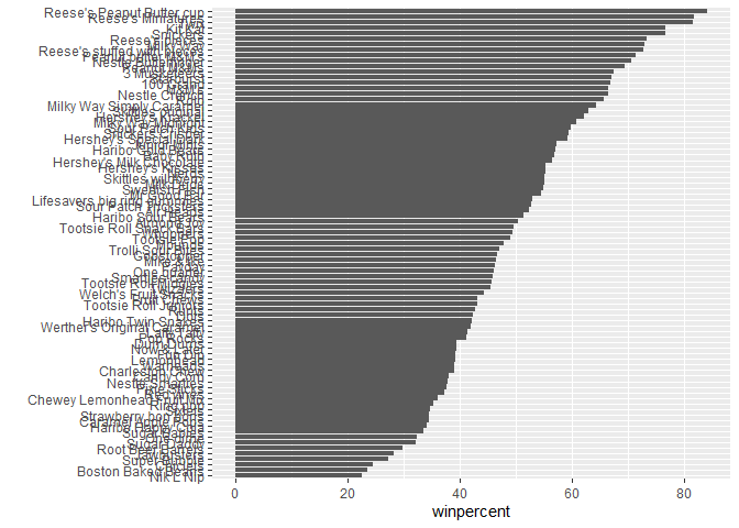
Q15. Make a first bar plot of candy ranking based on winpercent values.
ggplot(candy_file) +
  aes(winpercent, reorder(row.names(candy_file),winpercent)) +
  geom_col() + ylab("")
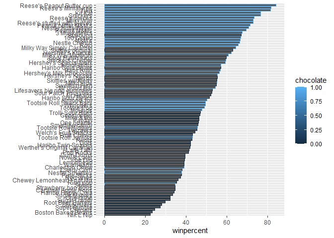
ggplot(candy_file) +
  aes(winpercent, reorder(row.names(candy_file),winpercent), col=chocolate) +
  geom_col() + ylab("")
We need a custom color vector
my_cols <- rep("black", nrow(candy_file))
my_cols[candy_file$chocolate==1] <- "chocolate"
my_cols[candy_file$bar==1] <- "brown"
my_cols[candy_file$fruity==1] <- "yellow"
my_cols
 [1] "brown"     "brown"     "black"     "black"     "yellow"    "brown"
 [7] "brown"     "black"     "black"     "yellow"    "brown"     "yellow"
[13] "yellow"    "yellow"    "yellow"    "yellow"    "yellow"    "yellow"
[19] "yellow"    "black"     "yellow"    "yellow"    "chocolate" "brown"
[25] "brown"     "brown"     "yellow"    "chocolate" "brown"     "yellow"
[31] "yellow"    "yellow"    "chocolate" "chocolate" "yellow"    "chocolate"
[37] "brown"     "brown"     "brown"     "brown"     "brown"     "yellow"
[43] "brown"     "brown"     "yellow"    "yellow"    "brown"     "chocolate"
[49] "black"     "yellow"    "yellow"    "chocolate" "chocolate" "chocolate"
[55] "chocolate" "yellow"    "chocolate" "black"     "yellow"    "chocolate"
[61] "yellow"    "yellow"    "chocolate" "yellow"    "brown"     "brown"
[67] "yellow"    "yellow"    "yellow"    "yellow"    "black"     "black"
[73] "yellow"    "yellow"    "yellow"    "chocolate" "chocolate" "brown"
[79] "yellow"    "brown"     "yellow"    "yellow"    "yellow"    "black"
[85] "chocolate"
Q16. This is quite ugly, use the reorder() function to get the bars sorted by winpercent?
ggplot(candy_file) +
  aes(winpercent, reorder(row.names(candy_file) ,winpercent)) +
  geom_col(fill = my_cols) + ylab("")
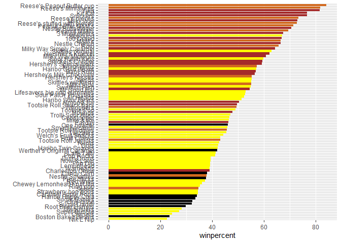
Q17. What is the worst ranked chocolate candy?
Nik L Nip
Q18. What is the best ranked fruity candy?
Reese’s Peanut Butter Cup
Taking a look at priceprint
library(ggrepel)

# How about a plot of win vs price

ggplot(candy_file) +
  aes(x = winpercent, y = pricepercent) + geom_point(col=my_cols) + geom_text_repel(col=my_cols, label=rownames(candy_file), size=3.3, max.overlaps = 5)
Warning: ggrepel: 54 unlabeled data points (too many overlaps). Consider
increasing max.overlaps
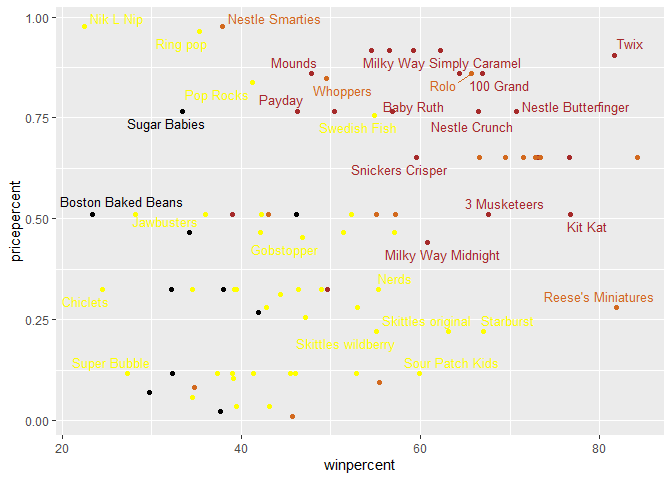
Q19. Which candy type is the highest ranked in terms of winpercent for the least money - i.e. offers the most bang for your buck?
Nik L Nip
Q20. What are the top 5 most expensive candy types in the dataset and of these which is the least popular?
ord <- order(candy_file$pricepercent, decreasing = TRUE)
head( candy_file[ord,c(11,12)], n=5 )
                         pricepercent winpercent
Nik L Nip                       0.976   22.44534
Nestle Smarties                 0.976   37.88719
Ring pop                        0.965   35.29076
Hershey's Krackel               0.918   62.28448
Hershey's Milk Chocolate        0.918   56.49050
Exploring the correlation data
cij <- cor(candy_file)
library(corrplot)
corrplot 0.95 loaded
corrplot(cij)
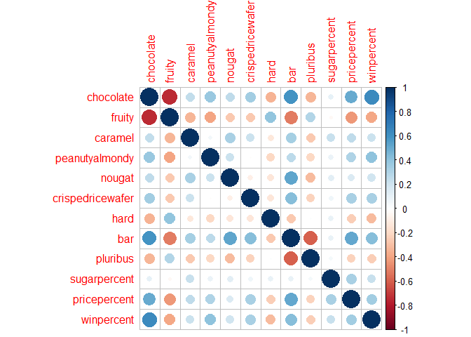
Q22. Examining this plot what two variables are anti-correlated (i.e. have minus values)?
Fruit and chocolate
Q23. Similarly, what two variables are most positively correlated?
Chocolate and bar
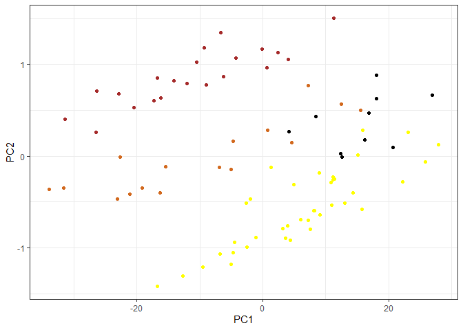
PCA
pca <- prcomp(candy_file)
summary(pca)
Importance of components:
                           PC1     PC2     PC3     PC4     PC5     PC6     PC7
Standard deviation     14.7231 0.70241 0.47762 0.37292 0.34641 0.33614 0.30748
Proportion of Variance  0.9935 0.00226 0.00105 0.00064 0.00055 0.00052 0.00043
Cumulative Proportion   0.9935 0.99574 0.99678 0.99742 0.99797 0.99849 0.99892
                           PC8     PC9    PC10    PC11    PC12
Standard deviation     0.27417 0.23826 0.21435 0.18434 0.15331
Proportion of Variance 0.00034 0.00026 0.00021 0.00016 0.00011
Cumulative Proportion  0.99927 0.99953 0.99974 0.99989 1.00000
ggplot(pca$x) +
aes(PC1, PC2, label=row.names(pca$x)) +
  geom_point(col=my_cols) + theme_bw()
ggplot(pca$rotation, aes(x = PC1, y = reorder(rownames(pca$rotation), PC1))) +
  geom_col()
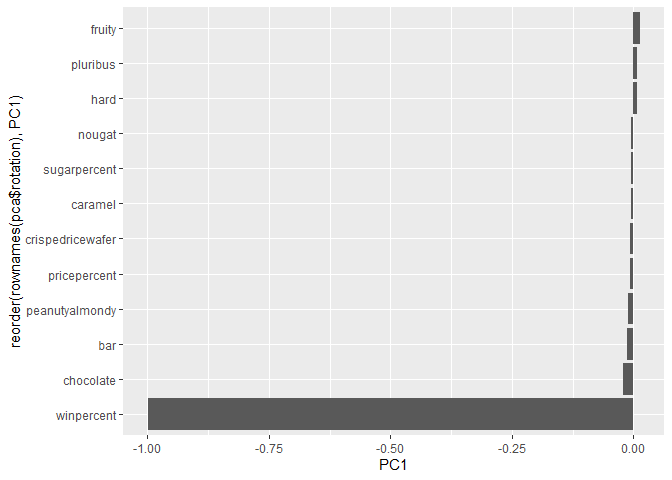
Q25. Based on your exploratory analysis, correlation findings, and PCA results, what combination of characteristics appears to make a “winning” candy? How do these different analyses (visualization, correlation, PCA) support or complement each other in reaching this conclusion?
It appears as though the analyses utilized within the lab showed that the strongest driving or winning candy are often moderately priced, chocolate-based and not fruity, and typically does include peanut and/or caramel. Reese’s peanut butter cup or general reese’s, Snickers, Twix, Kit Kat all sit right in this sweet spot, which is why they dominate winpercent.